Lecture 18: Spark Dataframes

Lecture 18: Spark Dataframes#

Learning Objectives#

By the end of this lecture, students should be able to:

Understand the concept of Resilient Distributed Datasets (RDDs) in Apache Spark.
Explain the immutability and fault tolerance features of RDDs.
Describe how RDDs enable parallel processing in a distributed computing environment.
Identify the key features of RDDs, including lazy evaluation and partitioning.

Introducing Spark DataFrames#

Like an RDD, a DataFrame is an immutable distributed collection of data. Unlike an RDD, data is organized into named columns, like a table in a relational database. Designed to make large data sets processing even easier

Spark DataFrames are a distributed collection of data organized into named columns, similar to a table in a relational database. They provide a higher-level abstraction than RDDs, making it easier to work with structured and semi-structured data. DataFrames support a wide range of operations, including filtering, aggregation, and joining, and they are optimized for performance through the Catalyst query optimizer. This makes them a powerful tool for big data processing and analytics.

What makes a Spark DataFrame different from other dataframes such as pandas DataFrame is the distributed aspect of it, similar to the RDDs concept that we learned in the last lecture.

Suppose you have the following table stored in a Spark DataFrame:

ID	Name	Age	City
1	Alice	30	New York
2	Bob	25	Los Angeles
3	Charlie	35	Chicago
4	David	40	Houston

As a programmer, you will see, manage, and transform this table as if it was a single and unified table. However, under the hoods, Spark splits the data into multiple partitions across clusters.

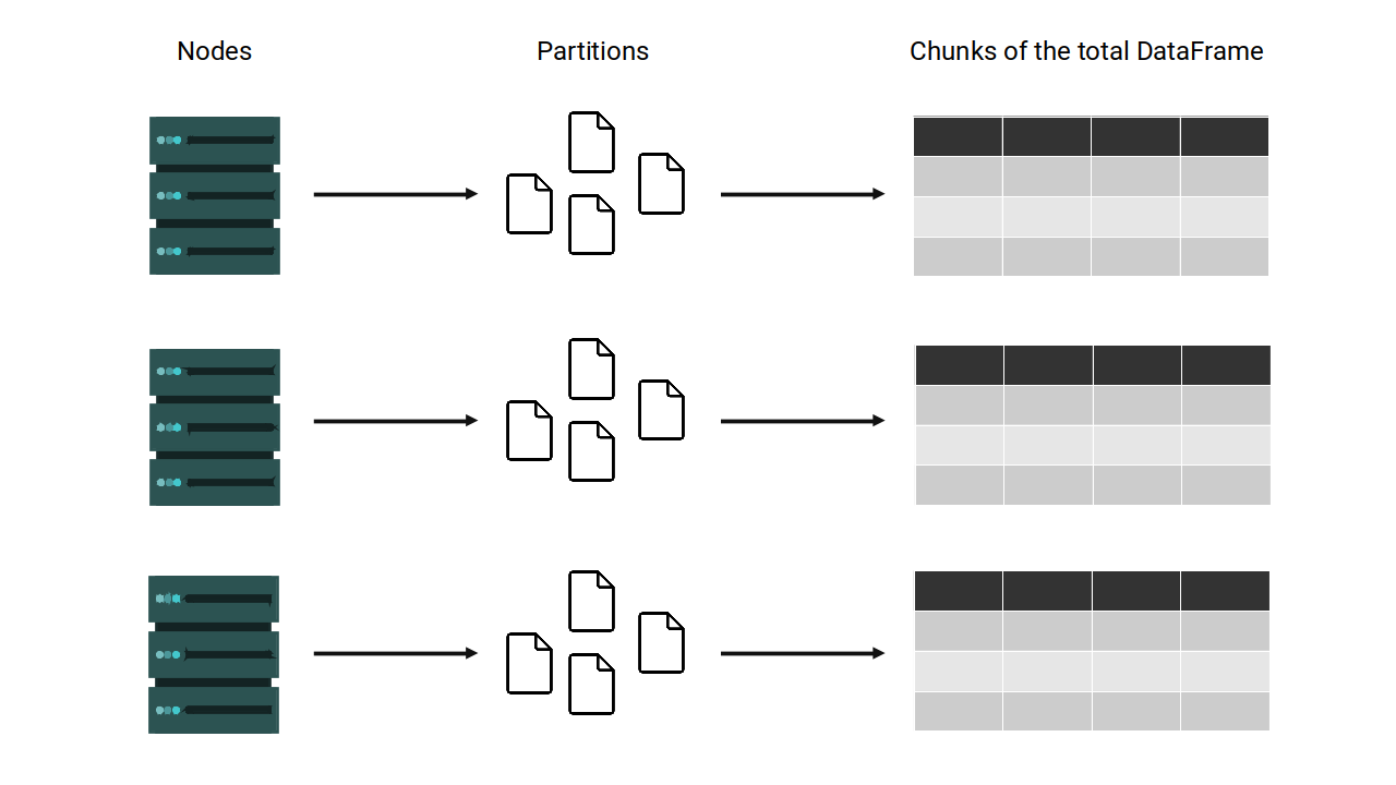
For the most part, you don’t manipulate these partitions manually or individually but instead rely on Spark’s built-in operations to handle the distribution and parallelism for you.

from pyspark.sql import SparkSession

# Initialize Spark Session
spark = SparkSession.builder \
    .master("local[1]") \
    .appName("DataFrame Example") \
    .getOrCreate()

spark

24/11/13 17:07:42 WARN Utils: Your hostname, Quans-MacBook-Pro.local resolves to a loopback address: 127.0.0.1; using 192.168.1.225 instead (on interface en0)
24/11/13 17:07:42 WARN Utils: Set SPARK_LOCAL_IP if you need to bind to another address
Setting default log level to "WARN".
To adjust logging level use sc.setLogLevel(newLevel). For SparkR, use setLogLevel(newLevel).
24/11/13 17:07:43 WARN NativeCodeLoader: Unable to load native-hadoop library for your platform... using builtin-java classes where applicable

SparkSession - in-memory

SparkContext

Spark UI

Version: v3.5.3
Master: local[1]
AppName: DataFrame Example

Create a `DataFrame` in `pyspark`#

Let’s create a sample spark dataframe

data = [("Alice", 34), ("Bob", 45), ("Cathy", 29)]
columns = ["Name", "Age"]

df = spark.createDataFrame(data, columns)
df

DataFrame[Name: string, Age: bigint]

Remember that a Spark DataFrame in python is a object of class pyspark.sql.dataframe.DataFrame as you can see below:

type(df)

pyspark.sql.dataframe.DataFrame

Let’s try to see what’s inside of df

df

DataFrame[Name: string, Age: bigint]

When we call for an object that stores a Spark DataFrame, Spark will only calculate and print a summary of the structure of your Spark DataFrame, and not the DataFrame itself.

To actually see the Spark DataFrame, you need to use the show() method.

df.show(2)

+-----+---+
| Name|Age|
+-----+---+
|Alice| 34|
|  Bob| 45|
+-----+---+
only showing top 2 rows

You can also show top n rows by using show(n)

df.show(2)

+-----+---+
| Name|Age|
+-----+---+
|Alice| 34|
|  Bob| 45|
+-----+---+
only showing top 2 rows

You could also display top n rows using the take() function, but the output is a list of Row objects, not formatted as a table.

df.take(2)

[Row(Name='Alice', Age=34), Row(Name='Bob', Age=45)]

Let’s get the name of the columns

df.columns

['Name', 'Age']

Let’s get the number of rows

df.count()

Data types and schema in Spark DataFrames#

The schema of a Spark DataFrame is the combination of column names and the data types associated with each of these columns

df.printSchema()

root
 |-- Name: string (nullable = true)
 |-- Age: long (nullable = true)

When Spark creates a new DataFrame, it will automatically guess which schema is appropriate for that DataFrame. In other words, Spark will try to guess which are the appropriate data types for each column.

You can create a dataframe with a predefined schema. For example, we want to set Age as integer

from pyspark.sql.types import StructType, StructField, StringType, IntegerType
from pyspark.sql import Row

schema = StructType([
    StructField("Name", StringType(), True),
    StructField("Age", IntegerType(), True)
])

data = [Row(Name="Alice", Age=30), Row(Name="Bob", Age=25), Row(Name="Charlie", Age=35)]

sample_df = spark.createDataFrame(data, schema)
sample_df.printSchema()

root
 |-- Name: string (nullable = true)
 |-- Age: integer (nullable = true)

Besides the “standard” data types such as Integer, Float, Double, String, etc…, Spark DataFrame also support two more complex types which are ArrayType and MapType:

ArrayType represents a column that contains an array of elements.

from pyspark.sql.types import StructType, StructField, StringType, ArrayType

# Define schema with ArrayType
schema = StructType([
    StructField("Name", StringType(), True),
    StructField("Hobbies", ArrayType(StringType()), True)
])

# Sample data
data = [
    ("Alice", ["Reading", "Hiking"]),
    ("Bob", ["Cooking", "Swimming"]),
    ("Cathy", ["Traveling", "Dancing"])
]

# Create DataFrame
df = spark.createDataFrame(data, schema)
df.show()

+-----+--------------------+
| Name|             Hobbies|
+-----+--------------------+
|Alice|   [Reading, Hiking]|
|  Bob| [Cooking, Swimming]|
|Cathy|[Traveling, Dancing]|
+-----+--------------------+

MapType represents a column that contains a map of key-value pairs.

from pyspark.sql.types import StructType, StructField, StringType, MapType

# Define schema with MapType
schema = StructType([
    StructField("Name", StringType(), True),
    StructField("Attributes", MapType(StringType(), StringType()), True)
])

# Sample data
data = [
    ("Alice", {"Height": "5.5", "Weight": "130"}),
    ("Bob", {"Height": "6.0", "Weight": "180"}),
    ("Cathy", {"Height": "5.7", "Weight": "150"})
]

# Create DataFrame
df = spark.createDataFrame(data, schema)
df.show()

+-----+--------------------+
| Name|          Attributes|
+-----+--------------------+
|Alice|{Height -> 5.5, W...|
|  Bob|{Height -> 6.0, W...|
|Cathy|{Height -> 5.7, W...|
+-----+--------------------+

Transformations of Spark DataFrame#

List of Transformations in Spark DataFrame

select()
filter()
groupBy()
agg()
join()
withColumn()
drop()
distinct()
orderBy()
limit()

data = [
    ("Alice", 34, "HR"),
    ("Bob", 45, "Engineering"),
    ("Cathy", 29, "HR"),
    ("David", 40, "Engineering"),
    ("Eve", 50, "Marketing"),
    ("Frank", 30, "Marketing"),
    ("Grace", 35, "HR")
]
columns = ["Name", "Age", "Department"]

df = spark.createDataFrame(data, columns)

1. `select`#

The select transformation is used to select specific columns from a DataFrame. It allows you to create a new DataFrame with only the columns you need.

Example:#

selected_df = df.select("Name", "Department")
selected_df.show()

+-----+-----------+
| Name| Department|
+-----+-----------+
|Alice|         HR|
|  Bob|Engineering|
|Cathy|         HR|
|David|Engineering|
|  Eve|  Marketing|
|Frank|  Marketing|
|Grace|         HR|
+-----+-----------+

2. `filter`#

The filter transformation is used to filter rows based on a condition. It returns a new DataFrame containing only the rows that satisfy the condition.

Example:#

filtered_df = df.filter(df["Age"] > 40)
filtered_df.show()

+----+---+-----------+
|Name|Age| Department|
+----+---+-----------+
| Bob| 45|Engineering|
| Eve| 50|  Marketing|
+----+---+-----------+

3. `groupBy` and `agg`#

The groupBy transformation is used to group rows based on the values of one or more columns. The agg transformation is used to perform aggregate operations on the grouped data.

Example:#

from pyspark.sql.functions import avg, count

grouped_df = df.groupBy("Department").agg(
    avg("Age").alias("Average_Age"),
    count("Name").alias("Employee_Count")
)
grouped_df.show()

DataFrame[Department: string, Average_Age: double, Employee_Count: bigint]

4. `withColumn`#

The withColumn transformation is used to add a new column or replace an existing column in a DataFrame. It takes the name of the column and an expression to compute the values for the column.

Example:#

from pyspark.sql.functions import col

new_df = df.withColumn("Age_Plus_One", col("Age") + 1)
new_df.show()

+-----+---+-----------+------------+
| Name|Age| Department|Age_Plus_One|
+-----+---+-----------+------------+
|Alice| 34|         HR|          35|
|  Bob| 45|Engineering|          46|
|Cathy| 29|         HR|          30|
|David| 40|Engineering|          41|
|  Eve| 50|  Marketing|          51|
|Frank| 30|  Marketing|          31|
|Grace| 35|         HR|          36|
+-----+---+-----------+------------+

Summary#

select: Select specific columns from a DataFrame.
filter: Filter rows based on a condition.
groupBy and agg: Group rows and perform aggregate operations.
withColumn: Add a new column or replace an existing column.

Actions in Spark DataFrame#

Here are some common actions in Spark DataFrame, grouped by similarity:

Show and Display
- show()
- head()
- first()
- take()
Aggregation and Statistics
- count()
Collection and Conversion
- collect()
- toPandas()
- toJSON()
Saving and Writing
- write()
- save()
- saveAsTable()

Show and Display#

1. `show()`#

The show() action displays the content of the DataFrame in a tabular format. By default, it shows the first 20 rows.

Example:#

df.show()

+-----+---+-----------+
| Name|Age| Department|
+-----+---+-----------+
|Alice| 34|         HR|
|  Bob| 45|Engineering|
|Cathy| 29|         HR|
|David| 40|Engineering|
|  Eve| 50|  Marketing|
|Frank| 30|  Marketing|
|Grace| 35|         HR|
+-----+---+-----------+

2. `head()`#

The head() action returns the first n rows of the DataFrame as a list of Row objects. By default, it returns the first row.

Example:#

df.head(3)

[Row(Name='Alice', Age=34, Department='HR'),
 Row(Name='Bob', Age=45, Department='Engineering'),
 Row(Name='Cathy', Age=29, Department='HR')]

3. `first()`#

The first() action returns the first row of the DataFrame.

Example:#

df.first()

Row(Name='Alice', Age=34, Department='HR')

4. `take()`#

The take() action returns the first n rows of the DataFrame as a list of Row objects, similar to head().

Example:#

df.take(3)

[Row(Name='Alice', Age=34, Department='HR'),
 Row(Name='Bob', Age=45, Department='Engineering'),
 Row(Name='Cathy', Age=29, Department='HR')]

Aggregation and Statistics#

1. `count()`#

The count() action returns the number of rows in the DataFrame.

Example:#

df.count()

Collection and Conversion#

1. `collect()`#

The collect() action returns all the rows of the DataFrame as a list of Row objects.

Example:#

df.collect()

[Row(Name='Alice', Age=34, Department='HR'),
 Row(Name='Bob', Age=45, Department='Engineering'),
 Row(Name='Cathy', Age=29, Department='HR'),
 Row(Name='David', Age=40, Department='Engineering'),
 Row(Name='Eve', Age=50, Department='Marketing'),
 Row(Name='Frank', Age=30, Department='Marketing'),
 Row(Name='Grace', Age=35, Department='HR')]

2. `toPandas()`#

The toPandas() action converts the DataFrame to a Pandas DataFrame.

Example:#

pandas_df = df.toPandas()
pandas_df

	Name	Age	Department
0	Alice	34	HR
1	Bob	45	Engineering
2	Cathy	29	HR
3	David	40	Engineering
4	Eve	50	Marketing
5	Frank	30	Marketing
6	Grace	35	HR

3. `toJSON()`#

The toJSON() action converts the DataFrame to a JSON string.

Example:#

json_rdd = df.toJSON()
json_rdd.collect()

['{"Name":"Alice","Age":34,"Department":"HR"}',
 '{"Name":"Bob","Age":45,"Department":"Engineering"}',
 '{"Name":"Cathy","Age":29,"Department":"HR"}',
 '{"Name":"David","Age":40,"Department":"Engineering"}',
 '{"Name":"Eve","Age":50,"Department":"Marketing"}',
 '{"Name":"Frank","Age":30,"Department":"Marketing"}',
 '{"Name":"Grace","Age":35,"Department":"HR"}']

Saving and Writing#

1. `write()`#

The write() action is used to write the DataFrame to external storage systems such as HDFS, S3, or local file systems.

Example:#

df.write.csv("output.csv")

2. `save()`#

The save() action is used to save the DataFrame to a specified path. It is similar to write() but provides more options for saving data.

Example:#

df.write.format("parquet").save("output.parquet")

Pivot operations#

Pivot operations in PySpark are used to transform rows into columns, which can be particularly useful for data summarization and analysis.

Columns to rows#

data = [
    ('Agnostic', 27, 34, 60),
    ('Atheist', 12, 27, 37),
    ('Buddhist', 27, 21, 30)
]
cols = ['religion', '<$10k', '$10k-$20k', '$20k-$30k']
religion = spark.createDataFrame(data, cols)
religion.show()

+--------+-----+---------+---------+
|religion|<$10k|$10k-$20k|$20k-$30k|
+--------+-----+---------+---------+
|Agnostic|   27|       34|       60|
| Atheist|   12|       27|       37|
|Buddhist|   27|       21|       30|
+--------+-----+---------+---------+

Stack Expression:

The stack function is used to convert multiple columns into rows. The stack function takes three arguments:

The number of columns to be unpivoted (in this case, 3).
Pairs of column names and their corresponding values.
The stack_expr variable contains the expression to unpivot the columns <$10k, $10k-$20k, and $20k-$30k into two new columns: salary_range and avg_salary.

from pyspark.sql.functions import expr
stack_expr = """
stack(3,
    '<$10k', `<$10k`,
    '$10k-$20k', `$10k-$20k`,
    '$20k-$30k', `$20k-$30k`
) AS (salary_range, avg_salary)
"""

longer_religion = religion\
    .select('religion', expr(stack_expr))

longer_religion.show()

+--------+------------+----------+
|religion|salary_range|avg_salary|
+--------+------------+----------+
|Agnostic|       <$10k|        27|
|Agnostic|   $10k-$20k|        34|
|Agnostic|   $20k-$30k|        60|
| Atheist|       <$10k|        12|
| Atheist|   $10k-$20k|        27|
| Atheist|   $20k-$30k|        37|
|Buddhist|       <$10k|        27|
|Buddhist|   $10k-$20k|        21|
|Buddhist|   $20k-$30k|        30|
+--------+------------+----------+

Rows to columns#

from pyspark.sql.functions import first
# Equivalent to the `religion` DataFrame:
longer_religion\
    .groupby('religion')\
    .pivot('salary_range')\
    .agg(first('avg_salary'))\
    .show()

+--------+---------+---------+-----+
|religion|$10k-$20k|$20k-$30k|<$10k|
+--------+---------+---------+-----+
|Agnostic|       34|       60|   27|
|Buddhist|       21|       30|   27|
| Atheist|       27|       37|   12|
+--------+---------+---------+-----+

Collecting and Expanding Operations#

In PySpark, collecting and expanding operations are useful for transforming and manipulating data, especially when dealing with nested structures or arrays.

Exploding#

The explode function is used to transform an array or map column into multiple rows. This is particularly useful when you have nested data and want to flatten it.

data = [
    (1, ["R", "Python"], {'dep': 'PR', 'name': 'Anne'}),
    (2, ["Scala"], {'dep': 'PM', 'name': 'Mike'}),
    (3, ["Java", "Python"], {'dep': 'HF', 'name': 'Sam'})
]
columns = ["employee_id", "knowledge", "employee_attrs"]
employees = spark.createDataFrame(data, columns)
employees.show()

+-----------+--------------+--------------------+
|employee_id|     knowledge|      employee_attrs|
+-----------+--------------+--------------------+
|          1|   [R, Python]|{name -> Anne, de...|
|          2|       [Scala]|{name -> Mike, de...|
|          3|[Java, Python]|{name -> Sam, dep...|
+-----------+--------------+--------------------+

When you apply the explode() function over a column of arrays, this function will create a new row for each element in each array it finds in the column

from pyspark.sql.functions import explode
explode_array = employees\
    .select(
        'employee_id',
        explode('knowledge')
    )

explode_array.show()

+-----------+------+
|employee_id|   col|
+-----------+------+
|          1|     R|
|          1|Python|
|          2| Scala|
|          3|  Java|
|          3|Python|
+-----------+------+

On the other hand, instead of arrays, the behaviour of explode() is slightly different when you apply it over a column of maps. Because each element in a map have two components: a key and a value.

As a consequence, when you apply explode() over a column of maps, each element in the map generates two different rows, which are stored in two separated columns, called key and value.

explode_map = employees\
    .select(
        'employee_id',
        explode('employee_attrs')
    )

explode_map.show()

+-----------+----+-----+
|employee_id| key|value|
+-----------+----+-----+
|          1|name| Anne|
|          1| dep|   PR|
|          2|name| Mike|
|          2| dep|   PM|
|          3|name|  Sam|
|          3| dep|   HF|
+-----------+----+-----+

This kind of output is powerful, specially with pivot operations, because you can easily organize all the data found in a column of maps into a series of new columns, like this:

explode_map\
    .groupby('employee_id')\
    .pivot('key')\
    .agg(first('value'))\
    .show()

+-----------+---+----+
|employee_id|dep|name|
+-----------+---+----+
|          1| PR|Anne|
|          2| PM|Mike|
|          3| HF| Sam|
+-----------+---+----+

Collecting#

The collect method is used to retrieve the entire DataFrame as a list of Row objects. This is typically used for small datasets due to memory constraints.

data = [
    (1, "Python"),
    (1, "SQL"),
    (2, "Java"),
    (2, "Scala"),
    (3, "Python"),
    (3, "Python"),
    (4, "Scala"),
    (4, "SQL")
]
explode_array = spark.createDataFrame(data, ["employee_id", "col"])
display(explode_array)

employee_id	col
1	Python
1	SQL
2	Java
2	Scala
3	Python
3	Python
4	Scala
4	SQL

In reverse, you can use the collect_list() and collect_set() functions to retract your DataFrame. That is, to reduce the number of rows of the DataFrame, while keeping the same amount of information.

The collect_list function collects all values in a column into an array, including duplicates.

from pyspark.sql.functions import collect_list

# Collecting all 'col' values into a list for each 'employee_id'
knowledge_list = explode_array.groupBy("employee_id").agg(collect_list("col").alias("knowledge_list"))
display(knowledge_list)

employee_id	knowledge_list
1	List(Python, SQL)
2	List(Java, Scala)
3	List(Python, Python)
4	List(Scala, SQL)

The collect_set function collects all unique values in a column into an array, removing duplicates.

from pyspark.sql.functions import collect_set

# Collecting unique 'col' values into a set for each 'employee_id'
knowledge_set = explode_array.groupBy("employee_id").agg(collect_set("col").alias("knowledge_set"))
display(knowledge_set)

employee_id	knowledge_set
1	List(Python, SQL)
2	List(Scala, Java)
3	List(Python)
4	List(Scala, SQL)

Lecture 18: Spark Dataframes

Contents

Lecture 18: Spark Dataframes#

Learning Objectives#

Introducing Spark DataFrames#

Create a DataFrame in pyspark#

Data types and schema in Spark DataFrames#

Transformations of Spark DataFrame#

1. select#

Example:#

2. filter#

Example:#

3. groupBy and agg#

Example:#

4. withColumn#

Example:#

Summary#

Actions in Spark DataFrame#

Show and Display#

1. show()#

Example:#

2. head()#

Example:#

3. first()#

Example:#

4. take()#

Example:#

Aggregation and Statistics#

1. count()#

Example:#

Collection and Conversion#

1. collect()#

Example:#

2. toPandas()#

Example:#

3. toJSON()#

Example:#

Saving and Writing#

1. write()#

Example:#

2. save()#

Example:#

Pivot operations#

Columns to rows#

Rows to columns#

Collecting and Expanding Operations#

Exploding#

Collecting#

Create a `DataFrame` in `pyspark`#

1. `select`#

2. `filter`#

3. `groupBy` and `agg`#

4. `withColumn`#

1. `show()`#

2. `head()`#

3. `first()`#

4. `take()`#

1. `count()`#

1. `collect()`#

2. `toPandas()`#

3. `toJSON()`#

1. `write()`#

2. `save()`#